Constituency, Substitution tests and the Inside-Outside Algorithm

A tale of a theory and an algorithm

One of the aspects that I like the most about NLP is connecting theories from linguistics to the models that we build and implement. In this post, I want to talk about one of the core notions of syntax, namely constituency, and see how one common test for constituency appears in computational models for syntax induction.

A brief overview of constituency

Briefly, a constituent is a group of words that together behaves as a single unit. For instance, in the sentence ‘the dog chases the cat’, we can rearrange ‘the dog’ and ‘the cat’ into ‘the cat chases the dog’, which is also an acceptable sentence. However, if we consider ‘the big red dog’, ‘red dog’ seems to be a constituent of the same type as ‘dog’, but ‘the big red’ doesn’t seem to be a constituent: while it would appear that ‘the’ is a substitutable word, most linguists do not accept ‘the’ as a constituent by itself.¹

Furthermore, constituents appear to be grouped together into different kinds: for example, whenever we see the phrase ‘the dog’ as a constituent, we can replace it with ‘the big red dog’ and still get a syntactically valid sentence. In fact, in both constituents, there appears to be a single word which expresses the general syntactic type of the constituent – that is, ‘dog’.

Together, these two empirical facts suggest a general test for constituency: if, for a given span of words, we can find a substitutable example from a common small set of examples, then that span is a constituent.² One common example is to use ‘it’ to substitute for noun phrases; another example is ‘do (so)’ for verb phrases. This test is known as the substitution test.³

Aside: why do constituents matter?

You may be wondering, dear reader, why we should care about the notion of constituency in the first place. I have two answers to this, one practical and one more scientific:

1. The scientific instinct to classify is strong, and constituency seems like a nice way to classify phrases into different kinds, and make generalisable statements about their syntactic behaviour.

2. Constituents, as a unit, often refer to things or events in the real world. If we are interested in more downstream application areas of language technology, such as information extraction, it is often useful to detect, e.g., the entities in the text.

Computational approaches towards constituency parsing

Now that we have an intuition about what a constituent is and why they are useful, let’s see how we can computationally induce constituents from text.

A formal model for constituency parsing: context-free grammars

First of all, we would like to introduce some rules for how we can analyse constituency. This framework should handle the fact that we can recursively combine words and pre-existing units into higher-level syntactic units, and that these syntactic units have types.

Context-free grammars (CFGs) are one commonly used framework. A context-free grammar consists of rules of the form \(A \to B C\), where \(A\), \(B\) and \(C\) are types of constituent, or rules of the form \(A \to w\) where \(A\) is a constituent type and \(w\) is a word. These grammars are called context-free because a rule only looks at the constituent \(A\) and not the surrounding context of the constituent. This is quite a strong assumption to make, and there is evidence that it may not be true for human language⁴, but remember: all models are wrong, some models are useful.

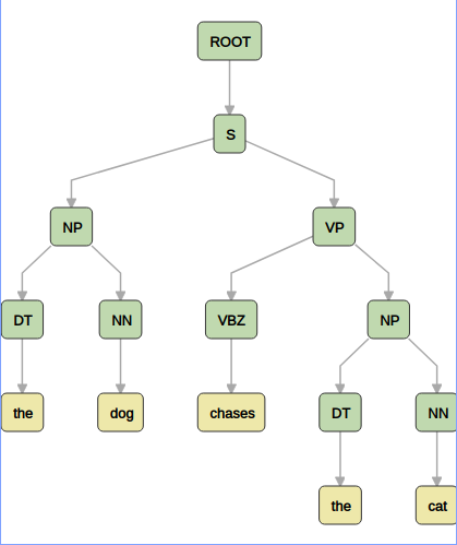
We’ve already seen one kind of constituent: ‘the dog’ is a noun phrase (\(\text{NP}\)). Other kinds of constituent are verb phrases (\(\text{VP}\)) and declarative clauses (\(\text{S}\), for some reason). One common example of a grammar rule is \(\text{S} \to \text{NP} \; \text{VP}\), which states that a declarative clause consists of a subject noun phrase and a predicate verb phrase.

Given a set of CFG rules, a parse for a sentence consists of a list of rule applications starting from some given root symbol, which produces the given sentence. See below for an example parse of our example sentence:

A constituency parse of the sentence 'the dog chases the cat', obtained from the CoreNLP parser. I highly recommend playing with it btw, see if you can break it!

At this point, you may have spotted that the way constituency is described is typically via a bottom-up merging process, while CFG production rules describe a top-down generating process. The parsing problem can therefore be thought of as inverting the CFG production process, starting at the end and trying to work back up to the root node. Due to the restrictive nature of CFG rules, we have access to efficient parsing algorithms which can enumerate all the possible parses of a given sentence. One example is the CYK algorithm. These algorithms progressively build up larger and larger subparses, starting from the words, until the full parse tree is built.

Ambiguity in parsing

One reason why language is hard is that language is inherently ambiguous in multiple ways. For example, ‘they can fish’ can either express the ability of an unspecified group of people to catch fish, or that said group of people put fish into metallic containers. Without more context, it is hard to tell which interpretation is preferable in this situation.

However, sometimes there can be clear preferences for one interpretation over another. Consider ‘they eat pizza with chopsticks’ vs. ‘they eat pizza with anchovies’. While superficially both sentences are similar, the correct interpretation for the latter sentence is that the pizza has the anchovies, whereas the eater has the chopsticks.

To deal with this kind of ambiguity, where multiple interpretations are possible, but some interpretations are more likely than others, it is useful to attach probabilities to the production rules of a CFG. This gives a probabilistic CFG, or PCFG. Now, every derivation of a sentence also comes with a score, obtained by multiplying the probabilities of the rules in the derivation. Ideally, we want to set the rule probabilities so that more likely interpretations have a higher score than unlikely interpretations (anchovies typically aren’t eating implements). But how do we do this?

Supervised constituency parsing

If we have annotated constituency information, we can frame constituency parsing as a supervised machine learning task. This is a long and noble line of work, and current supervised parsers reach human performance on in-domain data. However, I have always felt this is a slightly unsatisfying approach: we did not discover what a constituent was by looking at annotated constituency data. Is it possible to induce constituency structure directly from data without annotation?

Unsupervised constituency learning

Here is where the story gets interesting. Can we set up a model so that we just feed it raw text data and it spits out some notion of constituency? If we could design such a model, it would be very interesting:

1. For a start, it would be super impressive result: it always feels like magic to create something from nothing.
2. We could compare lots of different variants of such models in their ability to learn constituency. This would hopefully tell us something about the nature of constituency in human language.
3. Collecting annotated constituency data is expensive and time-consuming. If we could improve model performance by leveraging unannotated data, that would make our lives much easier.

One approach is to directly formalise the constituency tests that linguists propose into a computational model. This approach was taken by Steven Cao, Nikita Kitaev and Dan Klein at Berkeley in a very cool recent paper. However, in this post, I’ll look at unsupervised PCFG learning, and see how unsupervised PCFG learning procedures indirectly implement some linguistic constituency tests.

Unsupervised PCFG learning

Warning: here’s where the exposition becomes a bit more technical and maths-y.

Recall that a PCFG assigns a probability to a particular parse \(T\) of a sentence \(S\):

\[P(S, T) = \prod_{r \in T} P(r)\]

where each \(r\) is an instance of a CFG grammar rule, and \(P(r)\) is the probability of that rule, which is one of the parameters of the model (our complete model requires one of these parameters for every rule).

However, note that we can obtain the probability of a sentence \(S\) independent of any parse tree by summing over all possible parses for that sentence (this is called the marginal probability of \(S\)):

\[P(S) = \sum_T P(S, T)\]

Now, this gives us an objective function that does not refer to parse trees in any way. We can start off with an initial estimate of the probabilities \(P(r)\), and then try to maximise this resulting objective. However, how do we efficiently calculate the marginal probability above? The number of possible parses for a sentence is exponential in the sentence length, so the resulting sum could be over millions of possible parses.

However, just as there are efficient algorithms to enumerate all possible parses, there are efficient algorithms to calculate the marginal probability of a sentence. These algorithms all exploit the context-free nature of PCFGs, and iteratively build up probabilities of subsequences of the original sentence. Concretely, suppose \(S = w_0 w_1 \dots w_{n-1}\) is our sentence with words \(w_i\). Then, we will define, for a rule \(A \to B C\), the quantity

\[\alpha_{ij}(A) = P(A, w_i, \dots, w_j)\]

as denoting the probability of generating the span of words \(w_i, \dots, w_j\) starting from the constituent \(A\) and then applying the PCFG rules. Then, the overall probability of the sentence is given by \(\alpha_{0,n-1}(\text{ROOT})\). This quantity is known as the inside probability – roughly speaking, it tells you how likely a span of words is to be a constituent of type A. For example, the inside probability of ‘the dog’ to be an NP is high, whereas the inside probability of ‘the dog chases’ to be an NP is low.

The inside probability of A is the probability of generating the span from word i to word j starting from A, according to the PCFG rules. This figure suggests how we can calculate the inside probability efficiently by recursion. Figure from John Lafferty's notes on the inside-outside algorithm.

However, inside probabilities only tell half the story. Remember that our intuition about constituents did not come just from examining the constituent itself, but also the possible contexts of the constituent. For example, ‘chases the cat’ looks like a valid constituent, but ‘chases the cat chases the cat’ is an incoherent sentence (because the gap in ‘_ chases the cat’ expects a noun phrase, not a verb phrase).

We therefore need a quantity that captures the context of a constituent A. For this, we will define the outside probability, \(\beta_{ij}(A)\), as the probability that, starting from the root symbol, we can generate \(w_0, \dots, A, \dots, w_{n-1}\) (that is, A and all the words outside A, but not the words inside A). While there is a recursive definition of \(\beta_{ij}(A)\), one can also calculate it as the derivative of the total sentence likelihood w.r.t. the corresponding inside probability \(\alpha_{ij}(A)\) (see this Jason Eisner paper for more details).⁵

The outside probability of a constituent A is the probability of generating all the words outside of A, together with the constituent A (but not any of the contents of A). This figure shows how the outside probability can be calculated recursively using the inside probabilities and known outside probabilities, although we also need to consider the right hand side inside probabilities too. Figure again from John Lafferty's notes on the inside-outside algorithm.

Where does the substitution test come in?

I promised you at the start of the blog post that I’d connect the machine learning and the linguistics. Here is my attempt:

Remember the substitution test: two constituents are the same type if they are substitutable for each other in all contexts they appear in. We can therefore pick a set of canonical examples for each constituency type, and then test whether a span of words in a sentence is a constituent by substituting each of our canonical examples for that span, and seeing whether the result is a grammatical sentence.

Now, we’d like to search for the substitution test in PCFGs. We know that ‘gapped’ sentences correspond to outside probabilities, so the sentence-with-gap ‘_ chases the cat’ has associated with it an outside probability \(\beta(A)\) for each possible constituency type A. We also know for each of our canonical examples what type of constituent it is, so we know that, for instance, \(\alpha_{\text{it}}(NP) >> 0\) (we believe that ‘it’ is a likely noun phrase). If we now try to maximise the probability of the sentence ‘the dog chases the cat’, knowing that ‘it chases the cat’ is a highly probable sentence, what happens to the resulting inside and outside probabilities?

Well, since we know \(P(S) = \sum_A P(S, A) = \sum \alpha(A) \beta(A)\) (this statement says that we can generate a sentence by picking a constituent type A, generating what’s inside of A, what’s outside of A, and then summing over all possible constituents A), we can see that

\[P(\text{it chases cats}) = \alpha_{\text{it}}(NP) \beta_{\text{_ chases cats}}(NP) + \sum_A \left (\alpha_{\text{it}}(A) \beta_{\text{_ chases cats}}(A) \right)\]

forces \(\beta_{\text{_ chases cats}}(NP)\) to be high. This is really cool, because it shows that the \(\beta\) probabilities in some sense ‘encode’ the substitution test: they determine what kinds of fillers a gapped sentence expects.

Now, let’s examine the probability of ‘the dog chases the cat’:

\[P(\text{the dog chases cats}) = \alpha_{\text{the dog}}(NP) \beta_{\text{_ chases cats}}(NP) + \sum_A \left (\alpha_{\text{the dog}}(A) \beta_{\text{_ chases cats}}(A) \right)\]

Again, by a similar line of reasoning, as we know that ‘_ chases the cat’ expects a noun phrase, \(\alpha_{\text{the dog}}(NP)\) should be high, and we’ve correctly identified that ‘it’ and ‘the dog’ are both likely to be noun phrases in our simple model of constituency. Isn’t this neat?

As a bonus, the \(\beta\) probabilities naturally fall out of the learning process for unsupervised PCFGs, and they encode a test by which we as humans learnt about constituency. This suggests that, to learn about constituency, it’s not enough to just look at the contents of the constituent – one must also look at the surrounding context. I find this a neat parallel.

An Ending (Ascent)

Often, when we learn about algorithms in language processing, it’s a bit easy to get divorced from the fact that, actually, the algorithms are supposed to help us capture something fundamental about the way language works. I didn’t really understand the inside-outside algorithm until I realised how it encodes linguistic notions of constituency. I guess the main message I hope you, dear reader, take away is to always think about what we’re trying to study, and not lose sight of that when buried under mountains of mathematical notation.

A lot of the material in this blog post is firmly classical (i.e. pre-neural). Does anything carry over to the neural era? Well, while the inside-outside algorithm was originally developed for CFGs, the notion of combining content and context representations can be neuralised, and a really nice paper shows that the resulting structured neural algorithm also develops a very sophisticated notion of constituency from scratch.

Finally, recall that outside probabilities encode ‘gapped’ probabilities. If these seem familiar to you, that’s because gapped probabilities are fundamental in modern NLP as the masked language modelling objective that models like BERT use as a training objective. The big difference is that BERT does not make any independence assumptions to calculate these gapped probabilities, but I believe that it would be an interesting exercise to try to extract an unsupervised parser out of BERT.

---

Footnotes:

1. Whether ‘the’ is a constituent is a thorny issue. Another definition of a constituent is (roughly) something that can refer; under this definition, ‘the’ is not a constituent. ↩

2. Do all constituents have to be continuous spans of text? Some linguists allow the possibility of discontinuous constituents, and indeed there are efficient parsing algorithms for certain formalisms. ↩

3. There are also other tests for constituency, but in this post we will focus on the substitution test. ↩

4. Namely, CFGs cannot handle something called cross-serial dependencies which have been posited to exist in Dutch and Swiss German. ↩

5. Historically, the inside-outside algorithm was used to re-estimate the PCFG parameters during unsupervised learning. I always thought this was incomprehensible until I realised that all the inside-outside algorithm does is take gradient steps on the log-likelihood of a sentence until convergence, and that the outside algorithm naturally falls out of the gradient calculation. ↩